The ESPRESSO data reduction flow.¶

The ESPRESSO EDPS data reduction workflow removes the instrument signature from the raw science data. The workflow is written in Python and contains the classification and grouping rules, and the cascaded calls to the ESPRESSO pipeline recipes with the organization of the necessary transfers of files between them. The input files for each recipe are either unprocessed raw files or products from a previously completed recipes.

Recipes in the workflow are organized in a cascade, in order of execution. The overall data flow of the ESPRESSO pipeline is displayed here. The reduction cascade is organized in tasks (shown as rectangles with green-background labels on the top), which represent well-defined and usually self-contained steps in the process. Tasks can be grouped inside sub-workflows. Each task runs a recipe; the detailed description of the algorithms, inputs, outputs, and recipe parameters used in each recipe are available in the ESPRESSO Pipeline User Manual (see here for the latest version). Here we present only the most important features of the recipes and the workflow, or those features that are not covered in that manual.

The EDPS data reduction workflows process data in batches, called datasets, consisting of related science observations and the necessary calibrations. Therefore, the first steps in executing an EDPS data reduction workflow are to classify the input data and organize it into datasets. ESPRESSO follows the pattern adopted for many instruments designed for RV monitoring: each dataset includes only a single science observation (and all necessary calibrations for its processing) and each dataset is processed by the pipeline recipes separately, generating a product for each raw input file.

Next comes the processing of calibrations. Only those that are needed by the selected scientific exposures are processed.

Finally, the science data are processed and, as explained, a product is generated for each individual dataset, which is equivalent to a product for each individual raw science file. However, ESO provides a set of additional recipes grouped in ESO Tool Kit (ESOTK) that includes a recipe esotk_spectrum1d_combine designed to combine 1-dimensional spectra (in the ESO internal data product format; the ESPRESSO pipeline products are already in this format, so there is no need for conversion). The ESPRESSO EDPS workflow uses this recipe to generate a combined spectrum of multiple exposures. Whether or not the combined product is generated, depends on the selected Target Category: the default includes object and combine_science, the latter must be selected to carry out the combination; this target ensures that the combination is performed. This can be seen here in item 2a.

It is possible to set EDPS to perform the data reduction until a certain step of the reduction chain (e.g., to reduce only standard stars, or only flat fields). This is done by specifying the desired target in the field Select reduction target of the Raw Data tab.

Let’s consider the detailed structure of ESPRESSO sub-workflows. The rectangles representing each sub-workflow list on separate lines all tasks that they include, together with the main input data types and the name of the recipes that perform this reduction step, and any associated inputs and static calibrations that are necessary to fulfill these tasks. The arrow lines indicate the direction of the intermediate products’ transfer from one task/sub-workflow to another during the data processing.

The ESPRESSO reduction steps are:

1. Detector-level manipulations¶

The processing begins with the usual detector-related manipulations (bias, dark, detector monitoring), marked with the rectangle in the top row and performed in a separate sub-workflow. They include the following recipes: detmon_opt_lg_mr, espdr_mbias, espdr_mdark which derive the linearity correction, and produce master bias and dark, respectively. The first of these three recipes is not part of the ESPRESSO pipeline. It belongs to a specialized set of Detector monitoring recipes (DETMON) available from the usual ESO instrument pipeline
page, and has its own separate documentation.

Next, in another separate sub-workflow, the ESPRESSO EDPS workflow calls the recipes espdr_led_ff, espdr_orderdef, and espdr_mflat. They compute the gain and detect the bad pixels, define the locations of orders on the CCD (also called order tracing) and correct for the pixel-to-pixel sensitivity, respectively. The products from these and the previous recipes are used across the rest of the ESPRESSO workflow, as can be seen from the arrows that connect them with the following recipes and sub-workflows.

Go to top

2. Wavelength calibration¶

The wavelength calibration is performed in a separate sub-workflow. The workflow measures the cross-fiber contamination for the cases of Fabry-Pérot and ThAr lamp-illuminated fibers, computes the relative efficiency between sky and science fibers as a function of wavelength, and performs the actual wavelength calibration using the Fabry-Pérot etalon, the ThAr lamp, or the laser frequency comb (LFC), calling the recipes espdr_cal_contam, espdr_cal_eff_ab, espdr_wave_FP, espdr_wave_THAR, and espdr_wave_LFC, respectively.

The workflow calls the recipe espdr_wave_THAR twice to derive the ThAr-based wavelength calibration – for frames where the FP and ThAr sources alternate illuminating fibers A and B. The structure of the workflow here is complex, and it reflects the fact that, to produce a wavelength solution the pipeline combines the Fabry-Pérot peaks and some strong but not saturated ThAr lines. This is the baseline wavelength calibration method.

There is an option of laser frequency comb-based wavelength calibration via the recipe espdr_wave_LFC. It is called twice, alternating the illumination of the A and B fibers with the FP and the LFC. The LFC is a preferable wavelength calibration method for programs aiming to obtain accurate radial velocities (RV), because ThAr lamps degrade with time, leading to larger RV scatter. However, the ThAr provides a first guess for deriving the LFC solution, which explains the sequence of recipes in the workflow. Further details about the ESPRESSO wavelength calibration can be found in the ESPRESSO Pipeline User Manual, Sec. 11.

Go to top

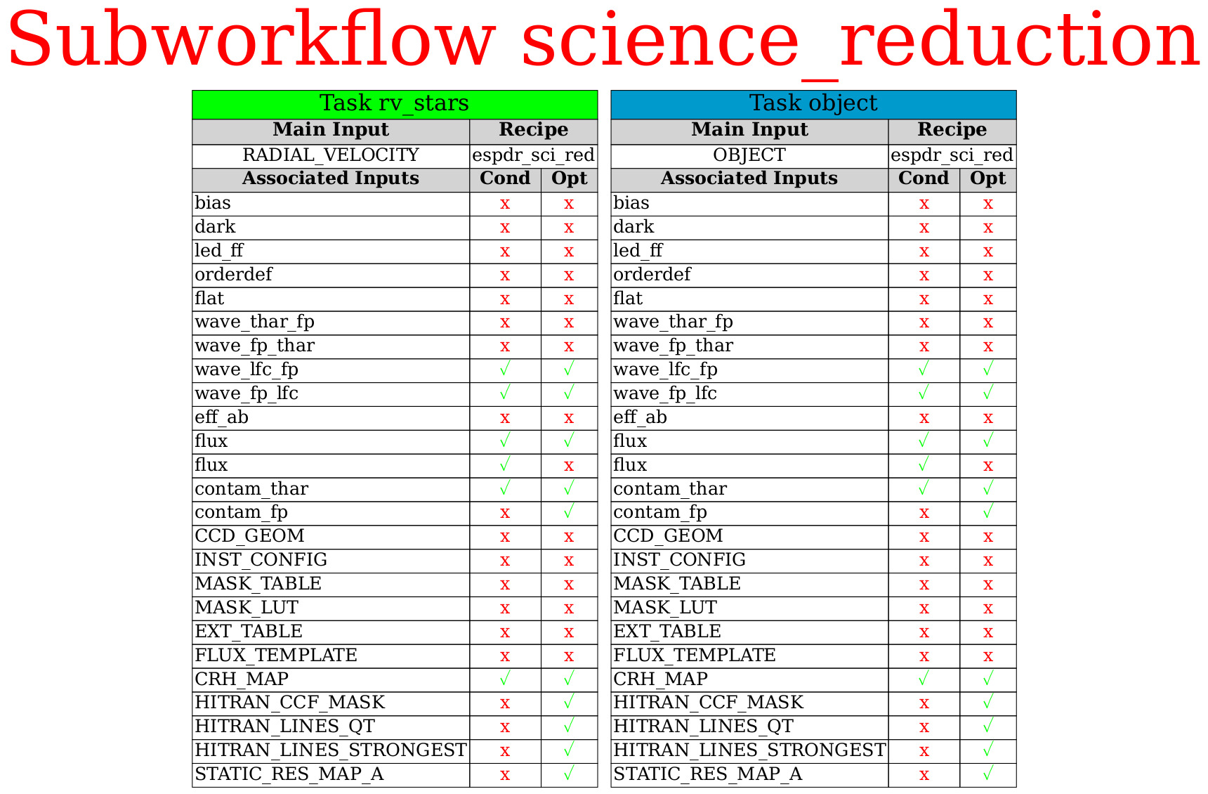
3. Science reduction¶

This includes the latest steps in the workflow diagram:

The flux calibration recipe espdr_cal_flux, that converts the flux of the science spectrum to ergs s−1 cm−2 A−1, based on a flux standard observation; it can also correct for the
extinction.
The science reduction recipe espdr_sci_red (in a sub-workflow of its own, called science reduction; it applies all calibrations to the science data, extracts the 1-dimensional spectra for all raw science frames, and calculates the RVs.
The ESOTK recipe esotk_spectrum1d_combine which combines together all 1-dimensional spectra that the ESPRESSO pipeline produced from science observations in the processed dataset. A detailed description of this recipe can be found in the ESOTK Pipeline User Manual. Importantly, this recipe propagates the errors, as appropriate.

Go to top

4. Pipeline products¶

EDPS saves the data products in $HOME/EDPS_data (default location; item 4 in Sec. Reducing demo data in this document explains how to change it). The first level of product sub-directories is by instrument, e.g., ESPRESSO in this case. The directory $HOME/EDPS_data contains a sub-directory graph with PDF files showing the instrument workflows - one shows a simplified overall workflow structure, others show the sub-workflows separately, and there is a plot that shows the workflow in its entirety.

The next sub-level of the directory structure contains directories organized by tasks. For ESPRESSO, these are: bias, combine_science, dark, eff_ab, flat, flux, led_ff, object, orderdef, wave_fp_fp, wave_fp_lfc, wave_fp_thar, wave_lfc_fp, and wave_thar_fp.

In turn, each of the sub-directories contains sub-directories on its own, corresponding to individual datasets, e.g., 44b1f5da-842e-44fe-95db-77661a23567d, 6e7a9f87-4342-45d7-9ba3-b33e19ee6131, b6db864b-ab35-4167-8c4a-3b11a4276f92, etc. These are different from the traditional timesstamp-type names that were used before, because EDPS is well suited for parallelization, and the latter may cause conflicts.

Each of the later sub-directories contain product FITS files, ASCII SOF files (with sets of input files) and ASCII RC files (with recipe parameters), various logs and a cmdline.sh file with the esorex command that was used to generate that particular product. This file can be executed from the command line:

    ./cmdline.sh

if the users want to reproduce the processing with the same SOF and RC files; the SOF and RC files can be edited, but this is recommended for expert users only. Note that the recipes use the default values for all parameters that are not listed in the rc files. For a full list of recipe parameters and their default values see the ESPRESSO pipeline user manual.

For each dataset and for each processing the pipeline stores the product files listed in Table 1. The file names start, by default, with the target name that is read from the ‘OBS TARG NAME’ keyword in the raw science file header. This keyword may contain spaces and they are carried over to the FITS file names. Some files are present among products only if the corresponding step in the reduction cascade was performed.

Table 1. An example of the ESPRESSO product spectra. Note the space in the file names which are carried over from the
‘OBS TARG NAME’ header keyword in the raw files.

Examples of FITS file product names	Category	Description
HD 10700_CCF_A.fits	CCF_A	CCF for fibre A with the object in S2D format. It contains the CCF for each order, with the corresponding errors and the data quality (in separate FITS extensions).
HD 10700_CCF_RESIDUALS_A.fits	CCF_RESIDUALS_A	Residuals from CCF computation of the RV for the spectrum – a FITS table with RVs, their errors and the residuals from the mean RV for each individual order of the spectrum.
HD 10700_DRIFT_MATRIX_B.fits	DRIFT_MATRIX_B	Drift matrix in S2D format with a single extension, storing the relative shift of the wavelength calibration solution position of the spectrum in fibre A (with the science target) relative to fibre B (with the calibration source) between the time of (night) observation and the time when the calibration was acquired (during the day).
HD 10700_S1D_A/B.fits	S1D_A/B	Extracted and merged 1d spectrum for fibre A/B (science target/calibr. or sky), stored in a FITS table with self-explanatory column names. The wavelength is in Å, the flux – in electrons or in physical units.
HD 10700_S1D_FINAL_A/B.fits	S1D_FINAL_A/B	Same as above but in an ESO Science Archive Phase III compatible format – some header keywords and column names are different, there are extra S/N columns.
HD 10700_S1D_FLUXCAL_A.fits	S1D_FLUXCAL_A	Flux calibrated spectrum for fibre A (target).
HD 10700_S2D_A/B.fits	S2D_A/B	Extracted and calibrated spectra by orders for fibre A/B (target/calibr. or sky). Useful for order-by-order inspection or processing.
HD 10700_S2D_BLAZE_A/B.fits	S2D_BLAZE_A/B	Blaze functions on order-by-order basis for fibre A/B.

More detailed descriptions of these files and their formats can be found in the ESPRESSO Pipeline User Manual.

In general, the ESPRESSO pipeline products follow two formats:

(1) S1D files are FITS tables that consist of a header with no data and a regular FITS table stored in the first extension (and can be inspected with any tool that reads FITS tables, such as topcat or fv). The column names in the table vary depending on the product type. Information about some columns that can be found in the S1D tables (e.g., in the S1D_FINAL_A files) is given in Table 2, and a plot of the S1D spectrum, generated with EDPS, is shown in the next figure:

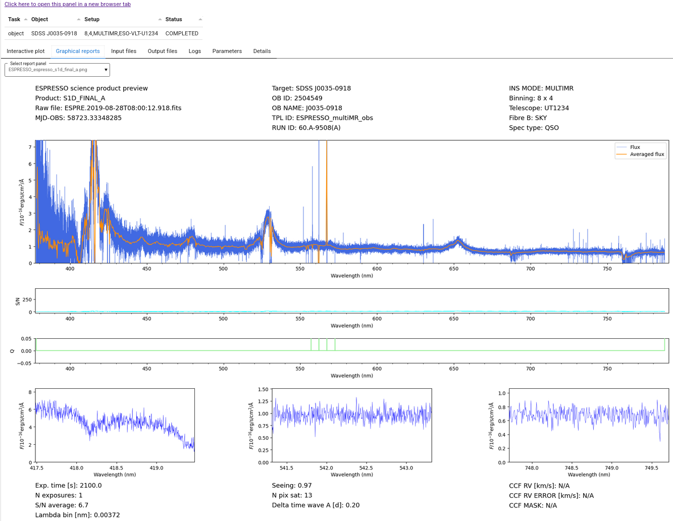
Table 2. An example of the ESPRESSO S1D product spectra.

Column name	Units	Description
WAVE	[Å]	Wavelength vector, in vacuum reference system.
FLUX	[erg cm−2 s−1 Å−1] or [e−]	Flux of the final extracted spectrum in Fibre A, fullyreduced till the end of the data reduction cascade. It is flux calibrated (if flux calibration was performed) and sky subtracted (if sky subtraction was performed).
ERR	[erg cm−2 s−1 Å−1] or [e−]	Error associated to FLUX.
QUAL		Quality flag associated to FLUX.
SNR		Signal to noise ratio, obtained from FLUX/ERR.
WAVE_AIR	[Å]	Wavelength vector, in the air reference system.
FLUX_EL	[e−]	Extracted flux from fibre A, not sky subtracted nor flux calibrated.
ERR_EL	[e−]	Error associated to FLUX_EL.
QUAL_EL		Quality flag associated to FLUX_EL.
FLUX_CAL	[erg cm−2 s−1 Å−1]	Extracted flux from fibre A, flux calibrated but not sky subtracted.
ERR_CAL	[erg cm−2 s−1 Å−1]	Error associated to FLUX_CAL.
QUAL_CAL		Quality flag associated to FLUX_CAL.
FLUX_CAL_SKYSUB	[erg cm−2 s−1 Å−1]	Extracted flux from fibre A, flux calibrated and sky subtracted.
ERR_CAL_SKYSUB	[erg cm−2 s−1 Å−1]	Error associated to FLUX_CAL_SKYSUB.
QUAL_CAL_SKYSUB		Quality flag associated to FLUX_CAL_SKYSUB.
FLUX_EL_SKYSUB	[e−]	Extracted flux from fibre A, sky subtracted by not flux calibrated.
ERR_EL_SKYSUB	[e−]	Error associated to FLUX_EL_SKYSUB.
QUAL_EL_SKYSUB		Quality flag associated to FLUX_EL_SKYSUB.

(2) S2D, CCF and blaze files are 2-dimensional images where each row corresponds to one extracted order (for ESPRESSO the number of extracted orders is 85-86). The S2D files consist of multiple extensions containing images of the same size that store wavelength (in vacuum and air, separately), flux, flux errors, data quality flags for each spectral element (extension name QUALDATA), and a few other parameters. The wavelength runs horizontally across the order, increasing from left to right, but it is stored in one of the extensions, so normally the files are displayed in pixels. The bluest orders are located at the bottom, and they are shorter than the reddest orders which are located on the top – this is due to the specifics of the ESPRESSO optical design. These files are 2-dimensional images, and they can be inspected with any image display tool such as fv or ds9. With the latter one can also plot cuts, and if the cuts are parallel to the lines, they will show the extracted spectra of the order corresponding to that line: to do this go to the Region pull-down menu, select the Shape item, then the Projection, and draw a line across the image. This plot will have pixels along the x-axis instead of wavelength. For more sophisticated treatment, or if the users want to analyze the data order by order, a programming approach is recommended, e.g., using Python.

S2D files can be inspected with any tool that displays 2-dimensional images, but analyzing individual orders requires programmatically extracting the wavelengths from one extension, the flux from another, and the errors - from a third.

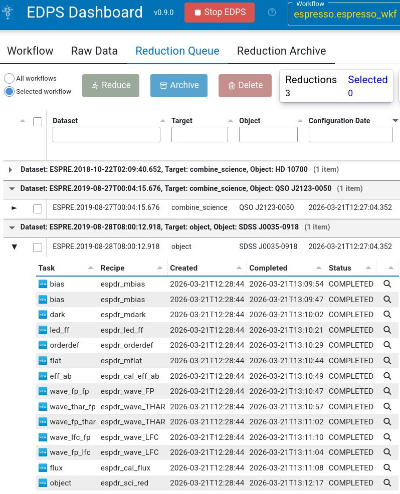
Plots of the S2D spectra are available in the EDPS as well. To produce such a plot, the users must go to the Reduction Queue, and click on the triangle (arrow) to the left of the dataset that they want to inspect. This will show the name of the input file (e.g., ESPRE.2019-08-28T08:00:12.918), again preceded by a triangle (arrow). Clicking on that triangle will show a table listing all the tasks that have been executed in the process of the reduction of that raw science frame. This will include bias, dark, led_ff, orderdef, flat, eff_ab, various wavelength steps, a flux calibration, and finally the object task. The users must press the magnifying glass symbol next to the object task to see a plot. This is illustrated in the next figure:

This plot is available by default when the Interactive Plot option is selected. The users can choose other options, including inspecting the input and output files, to see the pipeline produced logs or the parameters that were used in this particular step (by default, only the modified parameters are listed; click on All Parameters button to see them all).

For inspecting the products of other tasks or the input data the users instead of being shown a plot, will be offered access to some tools to open these FITS files, e.g. ds9 or fv.

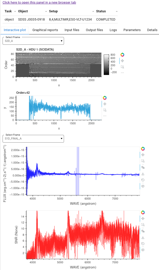
Finally, an example of an S2D plot is shown in the next plot. Note the pull-down menu Select Frame where one can select between different products. Further down in the same menu there are options to plot S1D spectra as well.

Inspection is important to carry out before the next step (archiving), to decide if the product satisfies the needs of the users. If this is not the case, the users may want to repeat the data processing with different parameter values. The parameter modification is described in the next section.

Once the users are satisfied with the data products, they can archive the products. This requires selecting the dataset that they are happy with and pressing the button Archive in the Reduction Queue tab. This will move that set to the Reduction Archive, as seen in the next figure:

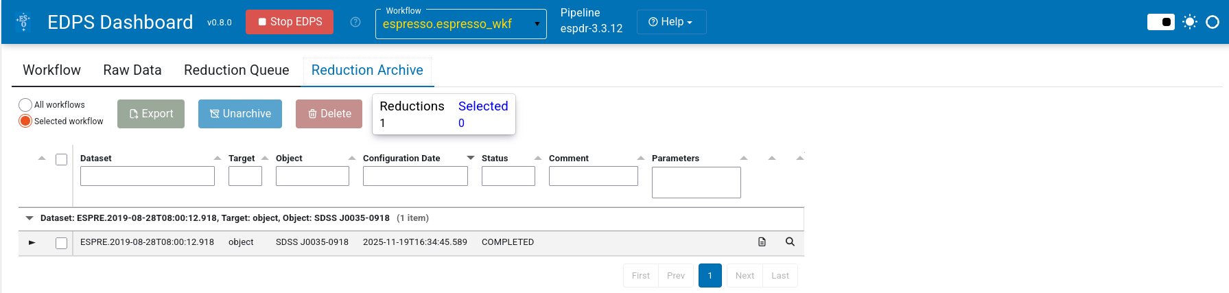
Already archived products can be removed from the archive with the button Unarchive - for example, if newer or better products are generated. Data products can also be deleted with the button Delete to free space.

It is also possible to save only the final products in a specified location, if the users are not interested in the intermediate products. This is done by exporting the archived data products: press the Export button in the Archived Data tab (see the figure above).

Go to top

Go to ESPRESSO EDPS tutorial index