Overview of all the data reduction configuration options 
Selection of most appropriate calibrations
By default, EDPS associates raw calibrations to the reduction process. It is also possible to use pre-processed calibrations (a.k.a. master calibrations) if available, in order to speed up the reduction. The preference can be specified in the Raw Data tab, before creating the datasets (see here).
Possible values of the Calibration Preferences are:
raw_per_quality_level: At equal quality of reduction, association of raw calibrations is preferred. This is the default.
master_per_quality_level: At equal quality of reduction, association of master calibrations is preferred.
raw. Association of raw calibration is preferred, despite the quality of results.
master. Association of master calibration is preferred, despite the quality of results.
When master calibrations are used, the reduction step needed to process raw calibrations are not executed. The reduction then moves directly to the process of scientific exposures.
For example, if reduction speed for a quick check is preferred over a high quality reduction, one can select “master”. In this case, old master calibrations are associated even if there are raw calibrations closer in time (and therefore more likely to ensure better quality products).
The quality level that the selected calibrations deliver is indicated close to each dataset in the
Raw input tab, under the colum CalibLevel. CalibLevel=0 indicates that
calibrations that follow the rules of the instrument calibration plans have
been selected. The higher the number, the poorer the quality of the products.
More information on the application properties file can be found here.
More explanations on the concept of “association levels” can be found here.
Configuration of parameters: the configuration editor
The data reduction of each dataset can be configured according to the scientific needs using an appropriate configuration editor. This editor allows to configure the data reduction for a given dataset by specifying workflow and recipe parameters.
The EDPS workflows contain two types of parameters and they both have default values that can be modified to improve the data reduction.
Workflow parameters are global and they are applied to the entire workflow. They are accessible both in the
Raw Datatab, prior to the creation og a dataset, and in theReduction Configurationeditor, in theReduction queuetab. Note: some workflow parameters were already configured before creating the dataset and sending it to the reduction queue. Here, they can be changed again. Please, note that the parameters have an effect only on the files that are already in the dataset. If one specifies a parameter that should include extra files in the dataset (e.g., the inclusion of more calibrations), files are not added and the reduction might fail. If you need to change a parameter that modifies the dataset content, please go back to the Raw data tab and create a new dataset.Recipe parameters are specific to the individual recipes and can be configured per task. They are accessible in the
Reduction Configurationeditor, in theReduction queuetab.
To open the Reduction configuration editor, click on
the wheel button  next to the dataset you desire to configure the reduction for. A window with the
configuration editor appears as shown the figure below.
next to the dataset you desire to configure the reduction for. A window with the
configuration editor appears as shown the figure below.

Fig. 1 The Reduction Configuration editor.
The editor is divided into 4 parts, which can be accessed pressing the corresponding expansion arrow.
Current configuration It indicates the name of the selected configuration for a given dataset.

Other configurations It allows to specify other configurations, to which the changes shall be copied to.

Comment It allows to specify a comment to describe the configuration. It is possible to append or replace a comment. Comments can be changed on all configurations. It is possible to save the comment for the current configuration only, or for all the selected configurations.

Parameters
This window is visible allows to:
Select the parameter set. A pre-determined list of workflow parameters and recipe parameters for a given use case. For the majority of the cases, the “science” parameter set can be used.
Edit the workflow parameters. These are parameters that regulates the reduction strategy, e.g. whether to use a given calibration or not, or to trigger a certain reduction step. Note that if the changes imply that some files not in the dataset are needed, the reduction might fail. In case, go back to the raw data tab, edit the workflow parameters there, and recreate the datasets.
Edit the recipe parameters. These are parameters associated to the recipe of a given task. Note: the same recipe parameters can be configured differently for the tasks that run the same recipe. Default parameters are shown (albeit some parameters can be dynamic, e.g.
EDPSchanges their value depending on the type of input data).
Change the values according to the needs and then select whether to save it to the current or the selected configurations. Note, complete configurations cannot be modified, new configurations will be automatically created instead.

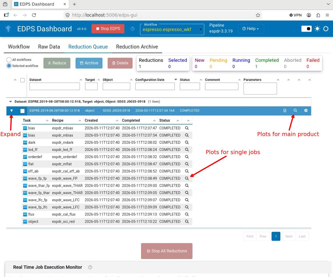
Quality reports
Almost all processing tasks can display the input raw frames and the products in the so called “quality plots”, which
can be inspected from the Reduction Queue window.
Those associated for the main product can be inspected by pressing the magnifying glass symbol at the right side of each dataset.
To inspect those associated to each individual job (if created),
Expand the desired dataset by pressing the black arrow on its left. The list of jobs will appear with the associated status (COMPLETED, RUNNING, PENDING)
Press the magnifying glass symbol at the right side of the job you want to inspect. Only plots for completed jobs can be inspected.
Radial Velocity Computation 
The ESPRESSO data reduction library contains a cross-correlation module that computes the cross-correlation function (CCF) of an S2D spectrum with respect to a binary template (mask) of a given spectral type. The radial velocity (RV) is then obtained from a Gaussian fit to the CCF. This technique has been successfully used on the ELODIE, CORALIE, HARPS, SOPHIE, and HARPS-N spectrographs (see Baranne et al. 1996, A&AS 119, 373, and Pepe et al. 2002, A&A 388, 632). One of its main advantages is that CCFs can be computed automatically using an absorption line mask. Line masks are simply lists of central wavelengths and depths of spectral lines, and can be created for various spectral types. We note here that the CCFs of slowly rotating stars are extremely well approximated by Gaussian profiles with a flat continuum. However, the particular fitting function does not matter much; the crucial aspect is to fit the CCFs of a given star always with the same function to avoid systematic effects on the derived radial velocities. As such, it is fundamental to reduce all the spectra with the same mask and CCF parameters, as comparisons between reductions with different parameters will be affected by systematics.
The main steps of the algorithm are:
(1) Compare the global flux distribution in the S2D spectrum to a static flux template that approximately corresponds to the spectral type of the star. The S2D flux is scaled accordingly to match the flux distribution of the template. In this way, spectra of any given star are always brought to the same flux distribution, which ensures that variable atmospheric conditions will not induce systematic effects in the CCF computation.
(2) Shift the wavelength scale of the S2D spectrum to the Solar-System barycenter using the barycentric correction.
(3) Define a uniform radial velocity grid that is approximately centered on the radial velocity of the star.
(4) For a given RV value in the grid, shift the line mask by the corresponding Doppler shift, project the line mask onto the S2D spectrum using a specified line width (about one pixel), and sum the S2D flux that goes through the so-defined mask holes. The flux from partial pixels is computed via simple linear interpolation. The sum is actually a weighted sum, using line depths as weights to optimally extract the Doppler information. During this process, the S2D spectrum is locally blaze corrected to remove any continuum slope around spectral lines. This produces one point of the CCF.
(5) Loop over all RV values in the grid.
(6) Fit a Gaussian profile to the CCF to derive RV, FWHM, and contrast.
Note that, by construction, CCFs are simply co-added spectral lines in velocity space, weighted by their depth and continuum flux, and corrected for the transmission of the grating (blaze function). As such they can be considered as a master spectral line for the star.
Go to top
Removal of cosmic rays 
Cosmic rays (CRs) are identified via a k-sigma rejection when extracting the one-dimensional spectrum from a single order. In each recipe that does it, the clipping is regulated by a dedicated parameter. In the science recipe, espr_sci_red the clipping is regulated by the parameter ksigma_cosmic. A value of -1 turns off the k-sigma clipping.
The science recipe has also an additional algorithm to detect CRs, that exploits L.A.Cosmic (van Dokkum 2001, PASP, 113, 1420). The algorithm is applied to the so-called detector-cleaned frames, i.e., the raw science where the overscan regions have been trimmed, and their contribution subtracted. Cosmics identified in this way are masked during the extraction of the one-dimensional spectra.
Both algorithms can be run simultaneously.
The L.A.Cosmic algorithm is regulated by the following parameters:
(1) cosmic_detection_sw: It turns L.A.Cosmic on (if set to 1) or off (if set to 0). By default, its value is taken by the input instrument configuration table. The algorithm is turned on for SKY mode, and it is turned off for FP-mode observations.
(2) lacosmic.post-filter-mode: dilate/dilute. It specifies whether CRs has to be dilated (i.e., expanded) or diluted (i.e., shrunk). It takes effect only if the post-filter-x/y values are positive.
(3) lacosmic.post-filter-x: X size of the post-filtering kernel. The mask is dilated or diluted by this amount along x-direction. Default: 0.
(4) lacosmic.post-filter-y: Y size of the post-filtering kernel. The mask is dilated or diluted by this amount along y-direction. Default: 0.
(5) lacosmic.sigma_lim: L.A.Cosmic Poisson fluctuation
threshold.
It is the minimum value of the fluctuation image, obtained by
dividing the Laplacian image (a second order derivative of the
original image along x and y) by the noise model. High values
of sigma_lim detect the more intense cosmics, and have
less risk of detecting false positives. Low values are more
efficient in finding also faint cosmics, but have a higher
risk of detecting false positives. The default values are
taken from the input instrument configuration table: 5
(SHR-SKY, 2x1), 7 (SHR-FP, 2x1), 7 (SHR 4x2), 8 (SUHR 1x1),
10 (MHR 4x2), 8 (MHR 8x6).
(6) lacosmic.f_lim: L.A.Cosmic minimum contrast between the Laplacian image (see above) and the fine-structure image (created from the original image by a combination of median filters). High values of f_lim detect the more intense cosmics, and have less risk of detecting false positives. Low values are more efficient in finding also faint cosmics, but have higher risk of detecting false positives. The default values are taken from the input instrument configuration table: 5 (SHR-SKY, 2x1), 5 (SHR-FP, 2x1), 5 (SHR 4x2), 8 (SUHR 1x1), 4 (MHR 4x2), 5 (MHR 8x6).
(7) lacosmic.max_iter: L.A.Cosmic maximum number of iterations; default: 5.
(8) extra_products_sw: Set to TRUE to create extra products to inspect L.A.Cosmic results; default: FALSE.
Go to top
Go to ESPRESSO EDPS tutorial index