The XSHOOTER data reduction flow
The overall data flow of the XSHOOTER pipeline is displayed here.
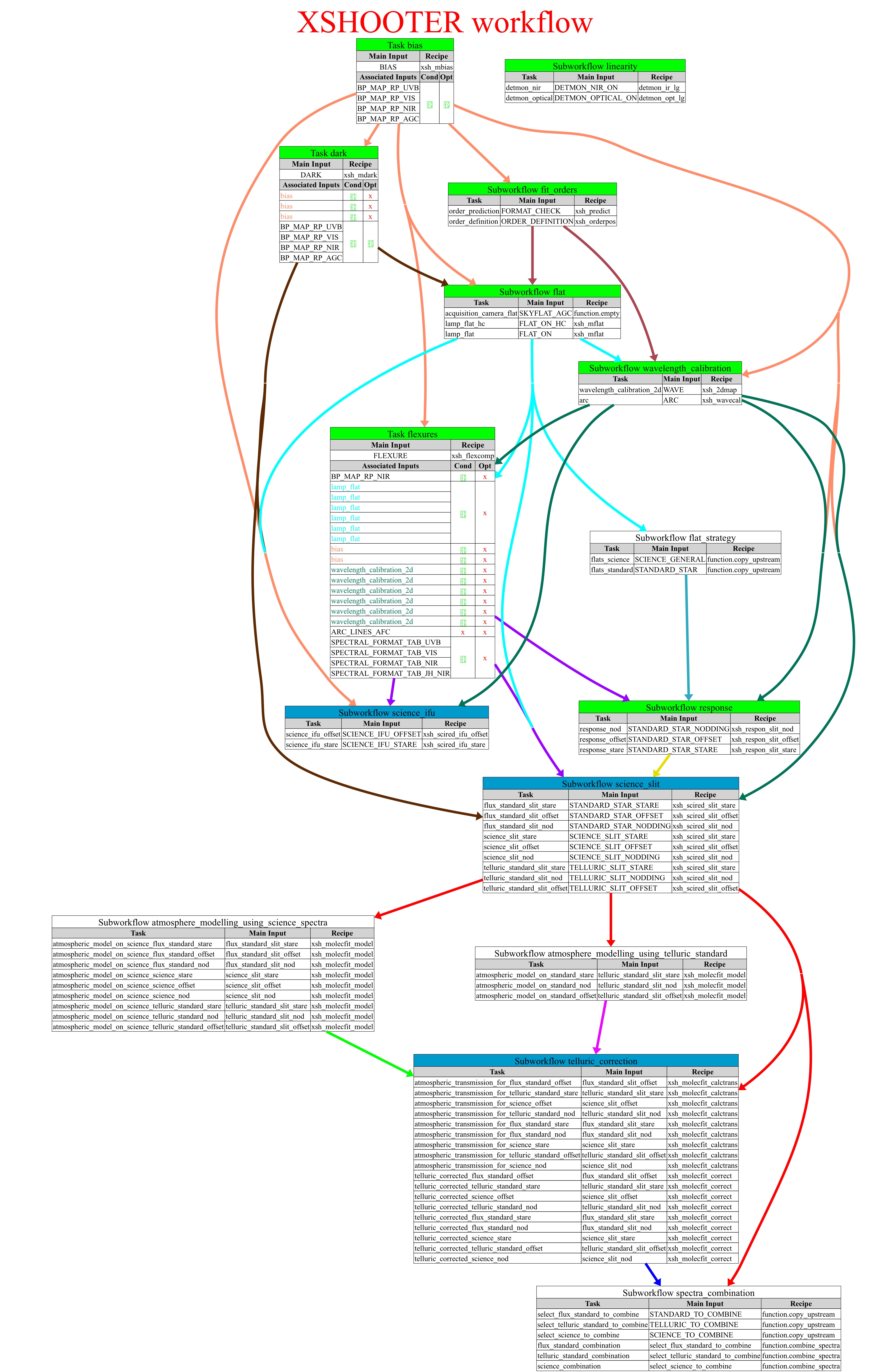
The reduction cascade is organized in tasks, which represent well-defined steps in the process. Tasks are grouped inside sub-workflows. Each task runs a recipe; the detailed description of the algorithms, input, outputs and recipe parameters used in each recipe are available in the pipeline manual. Here, we present only the description of the most important features.
The EDPS workflow is designed to execute the tasks that deliver
the final reduced spectrum (per order and merged) for each dataset,
optionally flux- and telluric-calibrated.
Only calibrations needed by the selected scientific exposures are processed.
It is possible to set EDPS to perform the data reduction until a certain step of the reduction chain
(e.g. to reduce only standard stars, or only flat fields).
This is controlled by the Select the reduction target option in the Raw Data tab.
The reduction steps are listed below. Before starting the reduction,
the parameters of the recipes associated to each task can be configured by pressing the button  close to each dataset configuration.
See here for more information.
close to each dataset configuration.
See here for more information.
1. Generate Master Bias
This step is carried in the task bias, which runs the recipe xsh_mbias.
Produces a master bias for UVB/VIS arms. NIR frames do not use bias frames.
Customization
Recipe parameters:
Choose stacking method (average, median) with
stack-method.Adjust sigma-clipping with
klowandkhigh.
2. Generate Master Dark
This step is carried in the task dark, which runs the recipe xsh_mdark.
Produces a master dark. Optional for UVB/VIS (dark current negligible). For NIR it is only needed for stare observations; generally not used in nodding/offset where ON–OFF subtraction removes the dark.
Customization
Recipe parameters:
Enable the use of darks for UVB/VIS data reduction with
use_optical_dark.Change
stack-methodandklow/khighthresholds to adjust stacking behaviour, e.g. for better cosmic-ray rejection.
3. Fit Orders
Computes initial guesses for the wavelength solution and order positions. Performed in two steps, described hereafter.
3a. Instrument Model Prediction
Recipe: xsh_predict
Uses the instrument physical model and information about ambient conditions during the observations (e.g. atmospheric pressure, temperature, instrument setting) to predict line positions and a first dispersion solution.
Customization
Workflow parameters:
Select between physical-model (recommended) and polynomial mode. See here for more information.
3b. Order Tracing (Determining Order Geometry)
Recipe: xsh_orderpos
Uses pinhole order-definition frames (ORDERDEF_*) to trace the location and curvature of each echelle order on the detector. Produces order tables that later help rectification and wavelength calibration.
Customization
Recipe parameters:
Tuning of detection thresholds can help when continuum levels are low or orders are partially vignetted.
4. Generate Master Flat
Recipe: xsh_mflat
Produces a master flat,
refined version of the table from xsh_orderpos
and a bad pixel map for each arm.
The flat defines the detector response and
updates the true geometry of the orders from slit illumination.
For IFU flat fields the edges of the slices are traced.
Customization
Recipe parameters:
Adjust bad-pixel handling (via
decode-bp) if master flats saturate or raise quality control errors.Change
stack-methodandklow/khighthresholds to adjust stacking behaviour, e.g. for better cosmic-ray rejection.
5. Wavelength Calibration
The wavelength calibration creates the wavelength and spatial resampling solutions and computes the arc-line tilts and instrumental resolution. It is done in two steps:
5a. 2D Mapping
Recipe: xsh_2dmap
Determines the two-dimensional wavelength solution needed to resample the orders.
Creates WAVE_TAB_2D_ARM,
which provides a full mapping from detector coordinates to wavelength+slit coordinates,
and SPECTRAL_FORMAT_TAB_ARM,
which defines, for each order, the wavelength range, pixel boundaries, predicted order edge traces,
and spatial-to-spectral coordinate conversion.
Customization
Workflow parameters:
Select between physical-model (recommended) and polynomial mode.
Recipe parameters:
Adjust line-detection thresholds for weak arcs via
detectarclines-fit-win-hsizeanddetectarclines-search-win-hsize. These parameters have to be small enough not to include a doublet but large enough to be able to detect and fit the line.
5b. Wavelength Calibration
Recipe: xsh_wavecal
Computes arc lines tilt and resolving power.
Customization
Workflow parameters:
Select between physical-model (recommended) and polynomial mode.
6. Flexure Compensation
Recipe: xsh_flexcomp
Refines the wavelength solution to account for flexure, especially when arcs are not taken at the same rotator angle as science.
Customization
Workflow parameters:
Select between physical-model (recommended) and polynomial mode.
7. Flat Strategy
This allows the user to choose between two strategies to select a flat field for the flux calibrator. The default strategy is to use the same flat as for the science observation. The alternative is to use the flat field selected by the rules, i.e., those taken closest in time to the flux calibrator.
Customization
Workflow parameters:
By default, the
use_flatparameter is set to science, meaning the flats used for science frames are also applied to standard stars. Set it to standard to use the flats taken closest in time to the standard-star observations.
8. Instrument Response and Efficiency
Recipes: xsh_respon_slit_stare, xsh_respon_slit_offset and xsh_respon_slit_nod
Use standard stars to derive the per-order and merged instrument response (mapping detector counts to physical flux), the blaze correction and the telescope + instrument + detector efficiency. Used for flux calibration of science exposures. The pipeline does not create response curves for IFU data, and they are therefore not flux-calibrated.
9. Science Reduction SLIT
Recipes: xsh_scired_slit_stare, xsh_scired_slit_offset and xsh_scired_slit_nod
Perform the data reduction:
Prepare the science frame (bias/dark/inter-order background correction, flat-fielding).
Rectify orders using the model and wavelength solution.
Perform sky subtraction (mode-dependent).
Localize the object and extract
ORDER1DandMERGE1Dproducts.
When several exposures are fed together,
the recipes stack them (mean/median) before extraction,
and you get one combined 2D and 1D spectrum per run, not one per exposure.
To obtain one spectrum per exposure (or per AB pair in nodding),
you must run xsh_scired_slit_* separately on each exposure or nod pair.
Customization
Workflow parameters:
By default,
telluric_correction_mode=standard derives the atmospheric parameters from the telluric standard. Set it to science to derive them directly from the science frame, or to none to disable telluric correction.Select between physical-model (recommended) and polynomial mode.
Recipe parameters:
Change
stack-methodandklow/khighthresholds to adjust stacking behaviour.Sky modelling: Use
sky-methodto select the method. In the NIR, BSPLINE2 provides the best residuals, BSPLINE1 is faster and acceptable for UVB/VIS, and MEDIAN is the fatest but may leave residuals.Sky region selection: use parameters
sky-position1,sky-hheight1,sky-position2, andsky-hheight2to manually select sky zones. Required when object not centered, multiple objects on slit, or strong NIR gradient.Spectroscopic extraction: Standard extraction (
localize-method=MANUAL) recommended for faint sources. Automatic detection (localize-method=AUTO) is usually fine for bright sources.
10. Science Reduction IFU (instrument mode decommissioned)
Recipes: xsh_scired_ifu_stare and xsh_scired_ifu_offset
Reduces a science IFU stare or on-off exposure and builds a 3D cube. Contrary to the slit mode, the pipeline does not create response curves for IFU data and they are therefore not flux-calibrated.
11. Atmospheric Modelling with Calibration Star
Recipe: xsh_molecfit_model
Models the atmosphere by fitting an atmospheric model to the input telluric-standard spectrum to derive the column densities of several molecular species.
The fitting process accounts for instrument-dependent parameters, including telescope background, spectral resolution, and wavelength calibration accuracy.
The products of this recipe are:
ATMOS_PARM: table containing atmospheric parameters (e.g. pressure, temperature, humidity),BEST_FIT_PARM: table with the best-fit atmospheric and instrumental parameters,BEST_FIT_MODEL: the best-fit atmospheric model to the data.
12. Atmospheric Modelling with Science
Recipe: xsh_molecfit_model
Same as step 11, but using the science spectrum to be corrected as input instead of a telluric-standard spectrum.
13. Telluric Correction
The telluric absorption correction is performed using the Molecfit software in two steps, as described below:
13a. Determine Correction
Recipe: xsh_molecfit_calctrans
Computes the telluric correction
by combining the atmospheric model produced by
xsh_molecfit_model with a single reduced observation
(science, flux standard, or telluric standard).
This step derives the atmospheric transmission over
the full wavelength range of the data.
If xsh_molecfit_model was computed using a different target
than the one processed by xsh_molecfit_calctrans
(e.g. a standard star instead of the science target),
the difference in airmass between the two observations
is taken into account when computing the transmission.
13b. Apply Correction
Recipe: xsh_molecfit_correct
Applies the telluric correction derived from the atmospheric transmission to the input data.
14. Spectra Combination
Recipe: esotk_spectrum1d_combine
This sub-workflow combines spectra selected according to the grouping rule
defined in the raw_spectra_to_combine datasource.
The process is performed in two steps:
first, the products of the relevant science reduction tasks are collected based on the raw frames;
second, the spectra are combined in a task named according to input_type.
The recipe used for the combination is esotk_spectrum1d_combine.
It resamples all input 1D spectra onto a common wavelength grid and stacks them.
It is well suited for combining a small number of spectra affected by cosmic rays,
using a median-based preprocessing step to identify and reject outliers;
for larger stacks, sigma clipping alone is usually sufficient.
15. Additional Tasks not used in the Science Reduction Cascade
15a. Detector Linearity
Recipes: detmon_opt_lg, detmon_ir_lg
These recipes identify pixels whose response to different flux levels deviates significantly from that of the majority of the detector (optical and infrared). Such pixels are flagged in the output mask with the value 32768 and are considered potential bad pixels. This step can be useful for diagnostic purposes, but is not strictly required and, by default, it is not included in the Reduction Cascade. The UVB/VIS detectors exhibit very few pixels of this type.
Go to XSHOOTER EDPS tutorial index