Overview of all the data reduction configuration options 
Selection of most appropriate calibrations
By default, EDPS associates raw calibrations to the reduction process. It is also possible to use pre-processed calibrations (a.k.a. master calibrations) if available, in order to speed up the reduction. The preference can be specified in the Raw Data tab, before creating the datasets (see here).
Possible values of the Calibration Preferences are:
raw_per_quality_level: At equal quality of reduction, association of raw calibrations is preferred. This is the default.
master_per_quality_level: At equal quality of reduction, association of master calibrations is preferred.
raw. Association of raw calibration is preferred, despite the quality of results.
master. Association of master calibration is preferred, despite the quality of results.
When master calibrations are used, the reduction step needed to process raw calibrations are not executed. The reduction then moves directly to the process of scientific exposures.
For example, if reduction speed for a quick check is preferred over a high quality reduction, one can select “master”. In this case, old master calibrations are associated even if there are raw calibrations closer in time (and therefore more likely to ensure better quality products).
The quality level that the selected calibrations deliver is indicated close to each dataset in the
Raw input tab, under the colum CalibLevel. CalibLevel=0 indicates that
calibrations that follow the rules of the instrument calibration plans have
been selected. The higher the number, the poorer the quality of the products.
More information on the application properties file can be found here.
More explanations on the concept of “association levels” can be found here.
Quality reports
Almost all processing tasks can display the input raw frames and the products in the so called “quality plots”, which
can be inspected from the Reduction Queue window.
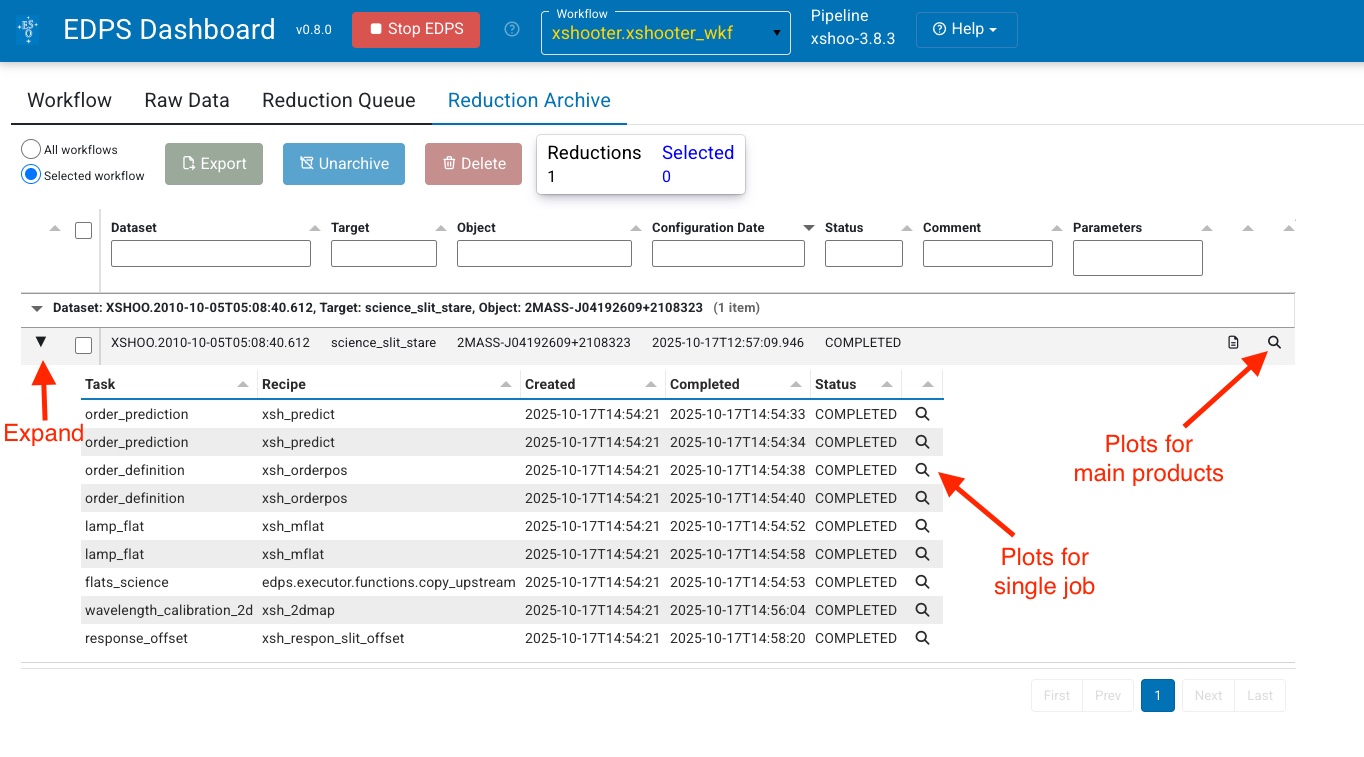
Those associated for the main product can be inspected by pressing the magnifying glass symbol at the right side of each dataset.
To inspect those associated to each individual job (if created),
Expand the desired dataset by pressing the black arrow on its left. The list of jobs will appear with the associated status (COMPLETED, RUNNING, PENDING)
Press the magnifying glass symbol at the right side of the job you want to inspect. Only plots for completed jobs can be inspected.
Configuration of parameters: the configuration editor
The data reduction of each dataset can be configured according to the scientific needs using an appropriate configuration editor. This editor allows to configure the data reduction for a given dataset by specifying workflow and recipe parameters.
The EDPS workflows contain two types of parameters and they both have default values that can be modified to improve the data reduction.
Workflow parameters are global and they are applied to the entire workflow. They are accessible both in the
Raw Datatab, prior to the creation og a dataset, and in theReduction Configurationeditor, in theReduction queuetab. Note: some workflow parameters were already configured before creating the dataset and sending it to the reduction queue. Here, they can be changed again. Please, note that the parameters have an effect only on the files that are already in the dataset. If one specifies a parameter that should include extra files in the dataset (e.g., the inclusion of more calibrations), files are not added and the reduction might fail. If you need to change a parameter that modifies the dataset content, please go back to the Raw data tab and create a new dataset.Recipe parameters are specific to the individual recipes and can be configured per task. They are accessible in the
Reduction Configurationeditor, in theReduction queuetab.
To open the Reduction configuration editor, click on
the wheel button  next to the dataset you desire to configure the reduction for. A window with the
configuration editor appears as shown the figure below.
next to the dataset you desire to configure the reduction for. A window with the
configuration editor appears as shown the figure below.
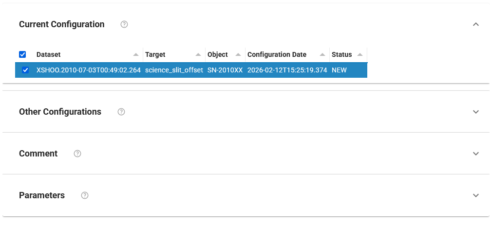
Fig. 7 The Reduction Configuration editor.
The editor is divided into 4 parts, which can be accessed pressing the corresponding expansion arrow.
Current configuration It indicates the name of the selected configuration for a given dataset.

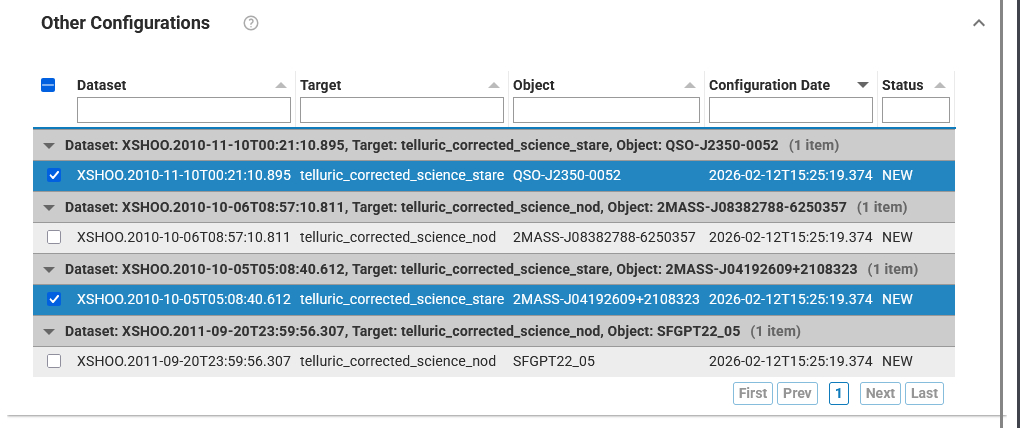
Other configurations It allows to specify other configurations, to which the changes shall be copied to.
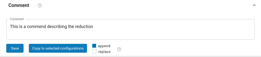
Comment It allows to specify a comment to describe the configuration. It is possible to append or replace a comment. Comments can be changed on all configurations. It is possible to save the comment for the current configuration only, or for all the selected configurations.
Parameters
This window is visible allows to:
Select the parameter set. A pre-determined list of workflow parameters and recipe parameters for a given use case. For the majority of the cases, the “science” parameter set can be used.
Edit the workflow parameters. These are parameters that regulates the reduction strategy, e.g. whether to use a given calibration or not, or to trigger a certain reduction step. Note that if the changes imply that some files not in the dataset are needed, the reduction might fail. In case, go back to the raw data tab, edit the workflow parameters there, and recreate the datasets.
Edit the recipe parameters. These are parameters associated to the recipe of a given task. Note: the same recipe parameters can be configured differently for the tasks that run the same recipe. Default parameters are shown (albeit some parameters can be dynamic, e.g.
EDPSchanges their value depending on the type of input data).
Change the values according to the needs and then select whether to save it to the current or the selected configurations. Note, complete configurations cannot be modified, new configurations will be automatically created instead.
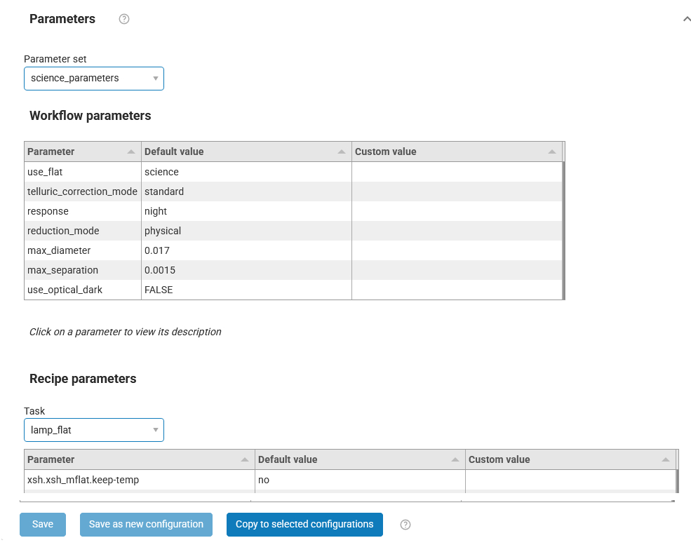
For XSHOOTER, the following workflow parameters can be adjusted
when the Target Category is set to science:
use_flat: By default, this parameter is set to science, meaning the flats used for science frames are also applied to standard stars. Set it to standard to use the flats taken closest in time to the standard-star observations instead.telluric_correction_mode: Atmospheric parameters can be derived either from a telluric standard or from the science frame itself. Set this parameter to standard (default) to use a telluric star observed the same night with the same instrument setup. Set it to science to derive the parameters directly from the science. Use none to disable telluric correction.response: This parameter selects the response curve used for flux calibration. night (default) uses the response from the standard star observed that night; if unavailable, fall back to the master response. master uses the master response from CalSelector, built by combining standards from multiple nights.reduction-mode: Select between the physical-model mode (recommended) and the polynomial mode to map each wavelength onto the CCDs. The physical model derives the solution from the actual optical path, while the polynomial method uses empirical multi-coefficient fits per order. If the reduction fails or the physical model appears inconsistent, the polynomial mode can be used for troubleshooting or as a fallback.max_diameter: TODOmax_separation: TODOuse_optical_dark: This parameter controls the use of a dark frame in the UVB/VIS data reduction. Because the dark current is negligible at these wavelengths, it is set to FALSE by default. Set it to TRUE if you wish to enable dark correction.
Troubleshooting 
This section provides guidance for diagnosing and resolving common issues encountered during the XSHOOTER data-reduction cascade.
Not enough arc lines detected 
The recipe xsh_2dmap may fail with an error indicating that not enough arc lines were detected.
Typical expected values for QC.NLINE.FOUND.CLEAN are:
UVB: ~2550 lines
VIS: ~3950 lines
NIR: ~1300 lines
Verify the quality and consistency of the input calibration products, in particular:
ARC_LINE_LIST_ARMTHEO_TAB_MULT_ARM(poly mode)ORDER_TAB_EDGES_SLIT_ARMWAVE_TAB_GUESS_ARM
In addition, adjust the line-detection parameters:
increase
detectarclines-search-winhsizedecrease
detectarclines-min-snto ensure more arc lines are detected.
Go to top
Sky subtraction residuals (especially NIR) 
Residual tilts between the sky model and the observed 2D frame can introduce sky–subtraction artefacts, particularly in the NIR. In practice, this manifests as alternating under- and over-subtracted regions around OH emission lines. See Figure Fig. 8 as an example.
Possible workarounds:
– #1 — Verify the accuracy of the xsh_2dmap products.
Run the reduction chain in physical-model mode,
which provides a more robust 2D geometry than the polynomial mode.
Ensure that the residuals after model optimisation are small;
if needed, re-run xsh_2dmap with additional iterations.
– #2 — Try setting sky-method = MEDIAN.
This can improve stability when the BSPLINE models fail
due to slight geometric mismatches.
– #3 — Apply flexure corrections computed by xsh_flexcomp.
Flexure compensation can realign the sky model and
reduce systematic sky–subtraction residuals.
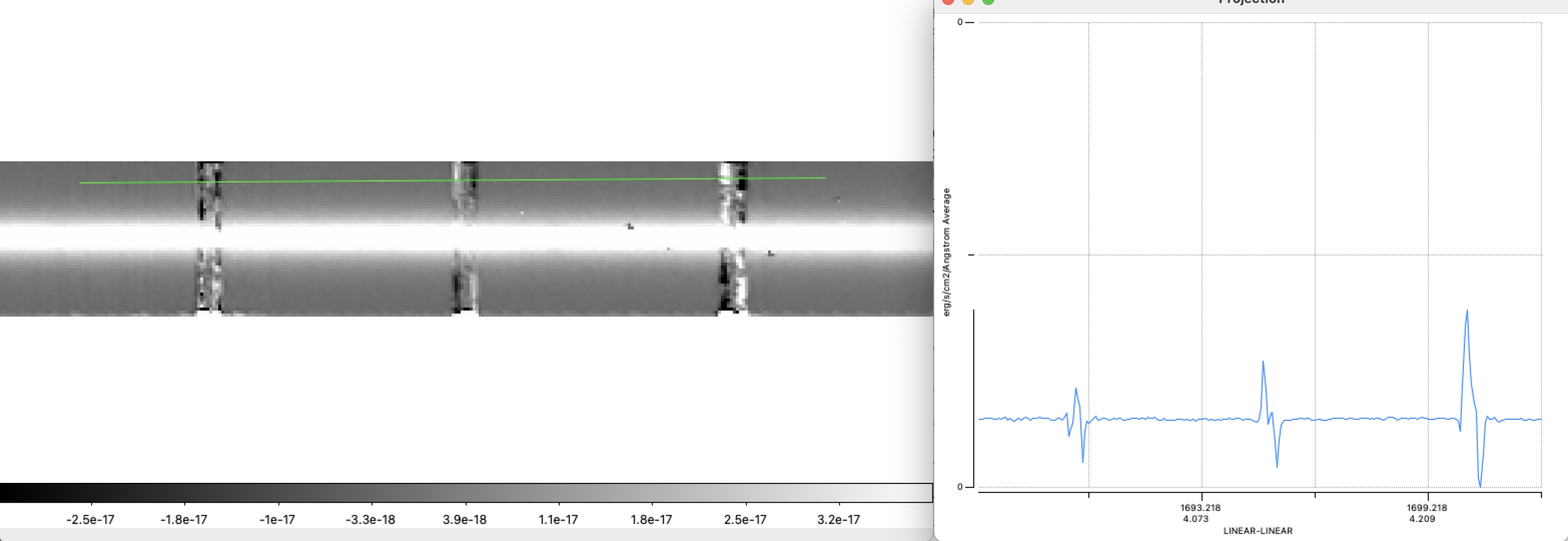
Fig. 8 Example of alternating under- and over-subtracted regions around OH emission lines, caused by a slight tilt of the sky lines relative to the object trace. The plot on the right shows the flux profile extracted along the green line in the 2D image.
Go to top
Trace-localization failures 
xsh_scired_slit_XXX may fail when extraction-method = LOCALIZATION
and localize-method is set to either GAUSSIAN or MAXIMUM.
This issue typically occurs with low S/N science exposures, where the object trace cannot be reliably detected using either the Gaussian cross-order profile or the maximum-detection algorithm.
The user should try adjusting
localize-slit-position and localize-slit-hheight
to guide the trace-localization process,
or alternatively set extraction-method = MANUAL,
which avoids automatic trace detection altogether.
Go to top
Two object traces in the slit 
Reduce each object trace separately by providing appropriate values in
the xsh_scired_slit_XXX recipe for the parameters
sky-position1, sky-hheight1, sky-position2, and sky-hheight2.
These parameters define the specific regions of the slit used
to estimate the sky during single-frame sky subtraction.
By default, all four parameters are set to zero, meaning that the sky is taken from all pixels outside the object localization region (and outside the masked slit edges). However, when multiple objects are present along the slit, or when the default choice is not appropriate, the user should manually adjust these positions.
Both the central positions and the half-heights of the sky regions are expressed in arcseconds.
Go to top
Order-edge artefacts in extracted spectra 
Artefacts may affect the edges of the 2D and 1D orders, degrading the quality of the merged extracted 2D and 1D spectra.
In such case, use the appropriate reference format-check frames
and verify that the values of
WLMIN and WLMAX in xsh_scired_slit_XXX are correct.
They should correspond to the last wavelength imaged
on the illuminated part of the order, divided by 1.007.
This can be checked by projecting the region files produced
by the script test_xsh_data_wave_tab_2d onto the
2D sky-subtracted science image.
Alternatively, in physical-model mode, the user may provide
a reference sky-line table (SKY_LINE_LIST_ARM)
and project the predicted sky-line positions onto
the 2D sky-subtracted frame to assess the consistency of order edges.
Go to top
Small jumps between orders 
Small discontinuities may appear between orders during merging,
typically caused by slit-edge artefacts introduced by the flat-field.
To mitigate this, we recommend setting extract-method = LOCALIZATION
in xsh_scired_slit_XXX.
For low S/N objects, use localize-method = MANUAL and
provide appropriate values for localize-slit-position and localize-slit-hheight.
For high S/N objects, localize-method = AUTO is generally sufficient.
Go to top
Overestimated uncertainties in the extracted spectrum 
This issue is typically caused by slit-edge artefacts introduced by the flat-field.
To mitigate it, set extract-method = LOCALIZATION in xsh_scired_slit_XXX
and choose an appropriate localization strategy:
For low S/N objects, use localize-method = MANUAL
and specify suitable values for
localize-slit-position and localize-slit-hheight.
For high S/N objects, localize-method = AUTO is usually sufficient.
Go to top
The extracted merged 1D spectrum looks poor 
The xsh_respon_slit_xxx and/or xsh_scired_slit_xxx recipes may have
failed to localize the trace correctly during extraction.
Try setting extract-method = LOCALIZATION and provide appropriate values
for localize-slit-position and localize-slit-hheight,
based on the appearance of the merged 2D spectral image
(e.g. SCI_SLIT_FLUX_MERGE2D_NIR.fits).
These parameters should be tuned so that:
the object lies near the centre of the extraction aperture, and
the extraction window fully includes the entire positive flux profile.
Go to top
Spectral regions of zero flux values 
Large regions of zero-flux values in the final extracted 1D spectrum may be caused by spurious Cosmic-Ray (CR) detections. See Fig. 9 as an example of affected spectrum.
CR-contaminated pixels are identified using the van Dokkum algorithm
(2001, PASP, 113, 1420)
applied to the input science frames.
The detection threshold is controlled by the parameter
removecrhsingle-sigmalim, whose default value is 5.0 for the UVB and VIS arms.
For the NIR arm, CR detection is disabled by default by setting
removecrhsingle-niter to 0.
In observations obtained under excellent seeing conditions (≈0.4″ or better),
the stellar PSF may appear sharp enough to be mistakenly flagged as CR-affected.
To reduce these false detections, increase the value of
removecrhsingle-sigmalim.
Figure Fig. 10 illustrates the improvement obtained on the same observation.
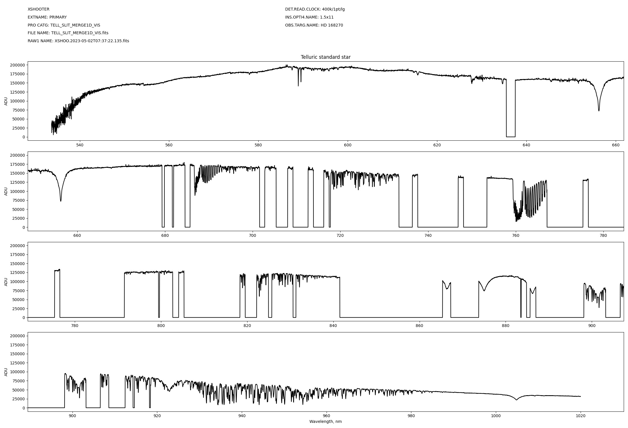
Fig. 9 Here we show the VIS spectrum of the telluric standard star Hip089684,
as displayed in the Graphical reports.
The observation was obtained on May 1, 2023
(OB identifier: XSHOO.2023-05-02T07:37:22.135)
under excellent seeing conditions (0.4″).
With the default value removecrhsingle-sigmalim=5.0,
the algorithm produces spurious cosmic-ray detections,
which in turn lead to extended wavelength intervals with zero flux
in the extracted 1D spectrum.
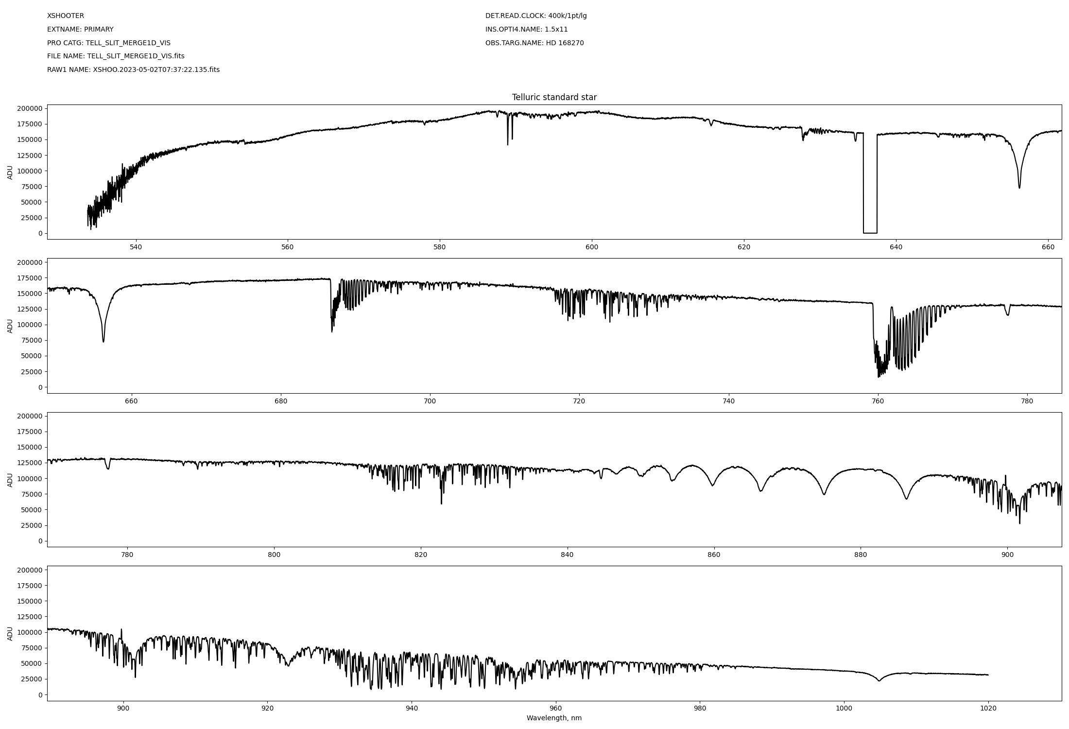
Fig. 10 Same as Fig. 9, but with removecrhsingle-sigmalim=7.0.
In this case, this avoids the flagging of good pixels as CR-affected.
IFU cube not well aligned 
Go to top
Go to XSHOOTER EDPS tutorial index